7. Tutorial: batch
hs_process.batch extends the functionality of the core modules of hs_process (segment, spatial_mod, and spec_mod) so that image processing can run via a relatively straightforward script without end user interaction.
The overall goal of the batch module is to implement many post-processing steps across many datacubes via an easy-to-use API. It was designed to save all data products (intermediate or final) to disk. Any unwanted files must be manually deleted by the user.
7.1. Sample data
Sample imagery captured from a Resonon Pika II VIS-NIR line scanning imager and ancillary sample files can be downloaded from this link.
Before trying this tutorial on your own machine, please download the sample files and place into a local directory of your choosing (and do not change the file names). Indicate the location of your sample files by modifying data_dir:
[1]:
data_dir = r'F:\\nigo0024\Documents\hs_process_demo'
7.2. Confirm your environment
Before trying the tutorials, be sure hs_process and its dependencies are properly installed. If you installed in a virtual environment, first check we are indeed using the Python instance that was installed with the virtual environment:
[2]:
import sys
import hs_process
print('Python install location: {0}'.format(sys.executable))
print('Version: {0}'.format(hs_process.__version__))
Python install location: C:\Users\nigo0024\Anaconda3\envs\hs_process\python.exe
Version: 0.0.4
The spec folder that contains python.exe tells me that the activated Python instance is indeed in the spec environment, just as I intend. If you created a virtual environment, but your python.exe is not in the envs\spec directory, you either did not properly create your virtual environment or you are not pointing to the correct Python installation in your IDE (e.g., Spyder, Jupyter notebook, etc.).
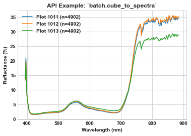
7.3. batch.cube_to_spectra
Calculates the mean and standard deviation for each cube in fname_list and writes the result to a “.spec” file. [API]
Note: The following batch example builds on the results of the `spatial_mod.crop_many_gdf tutorial <tutorial_spatial_mod.html#spatial_mod.crop_many_gdf>`__. Please complete the `spatial_mod.crop_many_gdf <tutorial_spatial_mod.html#spatial_mod.crop_many_gdf>`__ example to be sure your directory (i.e., base_dir) is populated with multiple hyperspectral datacubes. The following example will be using datacubes located in the following directory:
F:\\nigo0024\Documents\hs_process_demo\spatial_mod\crop_many_gdf
Load and initialize the batch module, checking to be sure the directory exists.
[3]:
import os
from hs_process import batch

base_dir = os.path.join(data_dir, 'spatial_mod', 'crop_many_gdf')
print(os.path.isdir(base_dir))
hsbatch = batch(base_dir, search_ext='.bip',
                progress_bar=True)  # searches for all files in ``base_dir`` with a ".bip" file extension
True
Use batch.cube_to_spectra to calculate the mean and standard deviation across all pixels for each of the datacubes in base_dir.
[4]:
hsbatch.cube_to_spectra(base_dir=base_dir, write_geotiff=False, out_force=True)
Processing file 39/40: 100%|████████████████████████████████████████████████████████████████████| 40/40 [00:02<00:00, 18.19it/s]
Use `seaborn <https://seaborn.pydata.org/index.html>`__ to visualize the spectra of plots 1011, 1012, and 1013. Notice how hsbatch.io.name_plot is utilized to retrieve the plot ID, and how the “history” tag is referenced from the metadata to determine the number of pixels whose reflectance was averaged to create the mean spectra. Also remember that pixels across the original input image likely represent a combination of soil, vegetation, and shadow.
[5]:
import seaborn as sns
import re
fname_list = [os.path.join(base_dir, 'cube_to_spec', 'Wells_rep2_20180628_16h56m_pika_gige_7_plot_1011-cube-to-spec-mean.spec'),
              os.path.join(base_dir, 'cube_to_spec', 'Wells_rep2_20180628_16h56m_pika_gige_7_plot_1012-cube-to-spec-mean.spec'),
              os.path.join(base_dir, 'cube_to_spec', 'Wells_rep2_20180628_16h56m_pika_gige_7_plot_1013-cube-to-spec-mean.spec')]
ax = None
for fname in fname_list:
    hsbatch.io.read_spec(fname)
    meta_bands = list(hsbatch.io.tools.meta_bands.values())
    data = hsbatch.io.spyfile_spec.load().flatten() * 100
    hist = hsbatch.io.spyfile_spec.metadata['history']
    pix_n = re.search('<pixel number: (.*)>', hist).group(1)
    if ax is None:
        ax = sns.lineplot(x=meta_bands, y=data, label='Plot '+hsbatch.io.name_plot+' (n='+pix_n+')')
    else:
        ax = sns.lineplot(x=meta_bands, y=data, label='Plot '+hsbatch.io.name_plot+' (n='+pix_n+')', ax=ax)
ax.set_xlabel('Wavelength (nm)', weight='bold')
ax.set_ylabel('Reflectance (%)', weight='bold')
ax.set_title(r'API Example: `batch.cube_to_spectra`', weight='bold')
[5]:
Text(0.5, 1.0, 'API Example: `batch.cube_to_spectra`')
7.4. batch.segment_band_math
Batch processing tool to perform band math on multiple datacubes in the same way. batch.segment_band_math is typically used prior to batch.segment_create_mask to generate the images/directory required for the masking process. [API]
Note: The following batch example builds on the results of the `spatial_mod.crop_many_gdf tutorial <tutorial_spatial_mod.html#spatial_mod.crop_many_gdf>`__. Please complete the `spatial_mod.crop_many_gdf <tutorial_spatial_mod.html#spatial_mod.crop_many_gdf>`__ example to be sure your directory (i.e., base_dir) is populated with multiple hyperspectral datacubes. The following example will be using datacubes located in the following directory:
F:\\nigo0024\Documents\hs_process_demo\spatial_mod\crop_many_gdf
Load and initialize the batch module, checking to be sure the directory exists.
[6]:
import os
from hs_process import batch

base_dir = os.path.join(data_dir, 'spatial_mod', 'crop_many_gdf')
print(os.path.isdir(base_dir))
hsbatch = batch(base_dir, search_ext='.bip',
                progress_bar=True)  # searches for all files in ``base_dir`` with a ".bip" file extension
True
Use batch.segment_band_math to compute the MCARI2 (Modified Chlorophyll Absorption Ratio Index Improved; Haboudane et al., 2004) spectral index for each of the datacubes in base_dir. See Harris Geospatial_ for more information about the MCARI2 spectral index and references to other spectral indices.
[7]:
folder_name = 'band_math_mcari2-800-670-550'  # folder name can be modified to be more descriptive in what type of band math is being performed
method = 'mcari2'  # must be one of "ndi", "ratio", "derivative", or "mcari2"
wl1 = 800
wl2 = 670
wl3 = 550
hsbatch.segment_band_math(base_dir=base_dir, folder_name=folder_name,
                          name_append='band-math', write_geotiff=True,
                          method=method, wl1=wl1, wl2=wl2, wl3=wl3,
                          plot_out=True, out_force=True)
Processing file 39/40: 100%|████████████████████████████████████████████████████████████████████| 40/40 [00:15<00:00, 2.59it/s]
batch.segment_band_math creates a new folder in base_dir (in this case the new directory is F:\\nigo0024\Documents\hs_process_demo\spatial_mod\crop_many_gdf\band_math_mcari2-800-670-550), which contains several data products.
The first is band-math-stats.csv: a spreadsheet containing summary statistics for each of the image cubes that were processed via batch.segment_band_math; stats include pixel count, mean, standard deviation, median, and percentiles across all image pixels.
[8]:
import pandas as pd

pd.read_csv(os.path.join(data_dir, 'spatial_mod', 'crop_many_gdf',
                         'band_math_mcari2-800-670-550', 'band-math-stats.csv')).head(5)
[8]:
| fname | plot_id | count | mean | std_dev | median | pctl_10th | pctl_25th | pctl_50th | pctl_75th | pctl_90th | pctl_95th | |
|---|---|---|---|---|---|---|---|---|---|---|---|---|
| 0 | F:\\nigo0024\Documents\hs_process_demo\spatial... | 1011 | 3391 | 0.622999 | 0.154441 | 0.647932 | 0.400957 | 0.526855 | 0.647932 | 0.743904 | 0.802663 | 0.825942 |
| 1 | F:\\nigo0024\Documents\hs_process_demo\spatial... | 1012 | 4902 | 0.627408 | 0.137226 | 0.651605 | 0.432411 | 0.545338 | 0.651605 | 0.732981 | 0.783473 | 0.806512 |
| 2 | F:\\nigo0024\Documents\hs_process_demo\spatial... | 1013 | 4902 | 0.483455 | 0.170385 | 0.491520 | 0.244630 | 0.349948 | 0.491520 | 0.626670 | 0.698892 | 0.737506 |
| 3 | F:\\nigo0024\Documents\hs_process_demo\spatial... | 1014 | 4902 | 0.582990 | 0.175643 | 0.618471 | 0.315483 | 0.473933 | 0.618471 | 0.727224 | 0.779835 | 0.804277 |
| 4 | F:\\nigo0024\Documents\hs_process_demo\spatial... | 1015 | 4902 | 0.582303 | 0.161018 | 0.597912 | 0.351104 | 0.461747 | 0.597912 | 0.716367 | 0.782069 | 0.809144 |
Second is a geotiff file for each of the image cubes after the band math processing. This can be opened in QGIS to visualize in a spatial reference system, or can be opened using any software that supports floating point .tif files.

Third is the band math raster saved in the .hdr file format. Note that the data conained here should be the same as in the .tif file, so it’s a matter of preference as to what may be more useful. This single band .hdr can also be opend in QGIS.
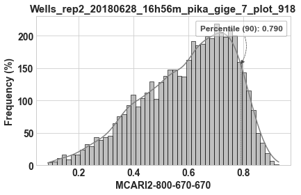
Fourth is a histogram of the band math data contained in the image. The histogram illustrates the 90th percentile value, which may be useful in the segmentation step (e.g., see `batch.segment_create_mask <tutorial_batch.html#batch.segment_create_mask>`__).
7.5. batch.segment_create_mask
Batch processing tool to create a masked array on many datacubes. batch.segment_create_mask is typically used after batch.segment_band_math to mask all the datacubes in a directory based on the result of the band math process. [API]
Note: The following batch example builds on the results of the `spatial_mod.crop_many_gdf tutorial <tutorial_spatial_mod.html#spatial_mod.crop_many_gdf>`__ and and `batch.segment_band_math <tutorial_batch.html#batch.segment_band_math>`__. Please complete both the spatial_mod.crop_many_gdf and batch.segment_band_math tutorial examples to be sure your directories (i.e., base_dir, and mask_dir) are populated with image files. The following example will be using
datacubes located in: F:\\nigo0024\Documents\hs_process_demo\spatial_mod\crop_many_gdf based on MCARI2 images located in: F:\\nigo0024\Documents\hs_process_demo\spatial_mod\crop_many_gdf\band_math_mcari2-800-670-550
Load and initialize the batch module, ensuring base_dir is a valid directory
[9]:
import os
from hs_process import batch

base_dir = os.path.join(data_dir, 'spatial_mod', 'crop_many_gdf')
print(os.path.isdir(base_dir))
hsbatch = batch(base_dir, search_ext='.bip',
                progress_bar=True)  # searches for all files in ``base_dir`` with a ".bip" file extension
True
There must be a single-band image that will be used to determine which datacube pixels are to be masked (determined via the mask_dir parameter). Point to the directory that contains the MCARI2 images.
[10]:
mask_dir = os.path.join(base_dir, 'band_math_mcari2-800-670-550')
print(os.path.isdir(mask_dir))
True
Indicate how the MCARI2 images should be used to determine which hyperspectal pixels are to be masked. The available parameters for controlling this are mask_thresh, mask_percentile, and mask_side. We will mask out all pixels that fall below the MCARI2 90th percentile.
[11]:
mask_percentile = 90
mask_side = 'lower'
Finally, indicate the folder to save the masked datacubes and perform the batch masking via batch.segment_create_mask
[12]:
folder_name = 'mask_mcari2_90th'
hsbatch.segment_create_mask(base_dir=base_dir, mask_dir=mask_dir,
                            folder_name=folder_name,
                            name_append='mask-mcari2-90th', write_geotiff=True,
                            mask_percentile=mask_percentile,
                            mask_side=mask_side, out_force=True)
Processing file 0/40:   0%|                                                                              | 0/40 [00:00<?, ?it/s]C:\Users\nigo0024\Anaconda3\envs\hs_process\lib\site-packages\spectral\io\spyfile.py:218: NaNValueWarning: Image data contains NaN values.
  warnings.warn('Image data contains NaN values.', NaNValueWarning)
Processing file 39/40: 100%|████████████████████████████████████████████████████████████████████| 40/40 [00:04<00:00,  8.28it/s]
batch.segment_create_mask creates a new folder in base_dir named according to the folder_name parameter (in this case the new directory is F:\\nigo0024\Documents\hs_process_demo\spatial_mod\crop_many_gdf\mask_mcari2_90th) which contains several data products.
The first is mask-stats.csv: a spreadsheet containing the band math threshold value for each image file. In this example, the MCARI2 value corresponding to the 90th percentile is listed.
[13]:
stats_fname = 'mask-{0}-pctl-{1}.csv'.format(mask_side, mask_percentile)
pd.read_csv(os.path.join(base_dir, 'mask_mcari2_90th', stats_fname)).head(5)
[13]:
| fname | plot_id | mask-lower-pctl-90-count | mask-lower-pctl-90-mean | mask-lower-pctl-90-stdev | mask-lower-pctl-90-median | |
|---|---|---|---|---|---|---|
| 0 | F:\\nigo0024\Documents\hs_process_demo\spatial... | 1011 | 339 | 0.832222 | 0.023752 | 0.826148 |
| 1 | F:\\nigo0024\Documents\hs_process_demo\spatial... | 1012 | 491 | 0.811119 | 0.021560 | 0.806518 |
| 2 | F:\\nigo0024\Documents\hs_process_demo\spatial... | 1013 | 491 | 0.743942 | 0.032975 | 0.737507 |
| 3 | F:\\nigo0024\Documents\hs_process_demo\spatial... | 1014 | 491 | 0.809495 | 0.022680 | 0.804289 |
| 4 | F:\\nigo0024\Documents\hs_process_demo\spatial... | 1015 | 491 | 0.813714 | 0.024030 | 0.809144 |
Second is a geotiff file for each of the image cubes after the masking procedure. This can be opened in QGIS to visualize in a spatial reference system, or can be opened using any software that supports floating point .tif files. The masked pixels are saved as null values and should render transparently.

Third is the full hyperspectral datacube, also with the masked pixels saved as null values. Note that the only pixels remaining are the 10% with the highest MCARI2 values.
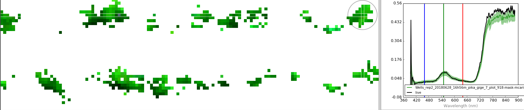
Fourth is the mean spectra across the unmasked datacube pixels. This is illustrated above by the green line plot (the light green shadow represents the standard deviation for each band).
7.6. batch.spatial_crop
Iterates through a spreadsheet that provides necessary information about how each image should be cropped and how it should be saved. [API]
If gdf is passed (a geopandas.GoeDataFrame polygon file), the cropped images will be shifted to the center of appropriate “plot” polygon.
Tips and Tricks for fname_sheet when gdf is not passed
If gdf is not passed, fname_sheet may have the following required column headings that correspond to the relevant parameters in `spatial_mod.crop_single <tutorial_spatial_mod.html#spatial_mod.crop_single>`__ and `spatial_mod.crop_many_gdf <tutorial_spatial_mod.html#spatial_mod.crop_many_gdf>`__:
“directory”
“name_short”
“name_long”
“ext”
“pix_e_ul”
“pix_n_ul”.
With this minimum input, batch.spatial_crop will read in each image, crop from the upper left pixel (determined as pix_e_ul/pix_n_ul) to the lower right pixel calculated based on crop_e_pix/crop_n_pix (which is the width of the cropped area in units of pixels).
Note: crop_e_pix and crop_n_pix have default values (see `defaults.crop_defaults <api/hs_process.defaults.html#hs_process.defaults>`__), but they can also be passed specifically for each datacube by including appropriate columns in fname_sheet (which takes precedence over defaults.crop_defaults).
fname_sheet may also have the following optional column headings:
“crop_e_pix”
“crop_n_pix”
“crop_e_m”
“crop_n_m”
“buf_e_pix”
“buf_n_pix”
“buf_e_m”
“buf_n_m”
“plot_id”
More fname_sheet Tips and Tricks
These optional inputs passed via
fname_sheetallow more control over exactly how the images are to be cropped. For a more detailed explanation of the information that many of these columns are intended to contain, see the documentation for`spatial_mod.crop_single<tutorial_spatial_mod.html#spatial_mod.crop_single>`__ and`spatial_mod.crop_many_gdf<tutorial_spatial_mod.html#spatial_mod.crop_many_gdf>`__. Those parameters not referenced should be apparent in the API examples and tutorials.If the column names are different in
fname_sheetthan described here,`defaults.spat_crop_cols<api/hs_process.defaults.html#hs_process.defaults>`__ can be modified to indicate which columns correspond to the relevant information.Any other columns can be added to
fname_sheet, butbatch.spatial_cropdoes not use them in any way.
Note: The following batch example only actually processes a single hyperspectral image. If more datacubes were present in base_dir, however, batch.spatial_crop would process all datacubes that were available.
Note: This example uses spatial_mod.crop_many_gdf to crop many plots from a datacube using a polygon geometry file describing the spatial extent of each plot.
Load and initialize the batch module, checking to be sure the directory exists.
[14]:
import os
import geopandas as gpd
import pandas as pd
from hs_process import batch

base_dir = data_dir
print(os.path.isdir(base_dir))
hsbatch = batch(base_dir, search_ext='.bip', dir_level=0,
                progress_bar=True)  # searches for all files in ``base_dir`` with a ".bip" file extension
True
Load the plot geometry as a geopandas.GeoDataFrame
[15]:
fname_gdf = os.path.join(data_dir, 'plot_bounds.geojson')
gdf = gpd.read_file(fname_gdf)
Perform the spatial cropping using the “many_gdf” method. Note that nothing is being passed to fname_sheet here, so batch.spatial_crop is simply going to attempt to crop all plots contained within gdf that overlap with any datacubes in base_dir.
Passing fname_sheet directly is definitely more flexible for customization. However, some customization is possible while not passing fname_sheet. In the example below, we set an easting and northing buffer, as well as limit the number of plots to crop to 40. These defaults trickle through to spatial_mod.crop_many_gdf(), so by setting them on the batch object, they will be recognized when calculating crop boundaries from gdf.
[16]:
import warnings

hsbatch.io.defaults.crop_defaults.buf_e_m = 2  # Sets buffer in the easting direction (units of meters)
hsbatch.io.defaults.crop_defaults.buf_n_m = 0.5
hsbatch.io.defaults.crop_defaults.n_plots = 40  # We can limit the number of plots to process from gdf

with warnings.catch_warnings():  # Suppresses the UserWarning that is issued
    warnings.simplefilter('ignore')
    hsbatch.spatial_crop(base_dir=base_dir, method='many_gdf',
                     gdf=gdf, out_force=True)
Because ``fname_list`` was passed instead of ``fname_sheet``, there is not a way to infer the study name and date. Therefore, "study" and "date" will be omitted from the output file name. If you would like output file names to include "study" and "date", please pass ``fname_sheet`` with "study" and "date" columns.
Processing file 39/40: 100%|████████████████████████████████████████████████████████████████████| 40/40 [00:03<00:00, 10.67it/s]
Processing file 39/40: 100%|████████████████████████████████████████████████████████████████████| 40/40 [00:03<00:00, 10.88it/s]
A new folder was created in base_dir - F:\\nigo0024\Documents\hs_process_demo\spatial_crop - that contains the cropped datacubes and the cropped geotiff images. The Plot ID from the gdf is used to name each datacube according to its plot ID. The geotiff images can be opened in QGIS to visualize the images after cropping them.
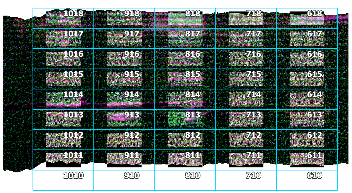
The cropped images were brightened in QGIS to emphasize the cropped boundaries. The plot boundaries are overlaid for reference (notice the 2.0 m buffer on the East/West ends and the 0.5 m buffer on the North/South sides).
7.7. batch.spectra_derivative
Calculates the numeric spectral derivative for each spectra in fname_list and writes the result as a “.spec” file. [API]
Note: The following batch example builds on the results of the `spatial_mod.cube_to_spectra tutorial <tutorial_batch.html#batch.cube_to_spectra>`__. Please complete both the `spatial_mod.crop_many_gdf <tutorial_spatial_mod.html#spatial_mod.crop_many_gdf>`__ and `spatial_mod.cube_to_spectra tutorial <tutorial_batch.html#batch.cube_to_spectra>`__ examples to be sure your directory (i.e., base_dir) is populated with multiple hyperspectral spectra. The following example will
be using spectra located in the following directory: F:\\nigo0024\Documents\hs_process_demo\spatial_mod\crop_many_gdf\cube_to_spec
Load and initialize the batch module, checking to be sure the directory exists.
[17]:
import os
from hs_process import batch

base_dir = os.path.join(data_dir, 'spatial_mod', 'crop_many_gdf', 'cube_to_spec')
print(os.path.isdir(base_dir))
hsbatch = batch(base_dir, search_ext='.spec', progress_bar=True)
True
Use batch.spectra_derivative to calculate the numeric spectral derivative for each of the .spec files in base_dir.
[18]:
hsbatch.spectra_derivative(base_dir=base_dir, out_force=True)
Processing file 39/40: 100%|████████████████████████████████████████████████████████████████████| 40/40 [00:01<00:00, 30.87it/s]
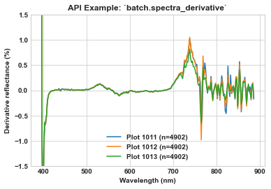
Use seaborn to visualize the derivative spectra of plots 1011, 1012, and 1013.
[19]:
import seaborn as sns
import re
fname_list = [os.path.join(base_dir, 'spec_derivative', 'Wells_rep2_20180628_16h56m_pika_gige_7_plot_1011-spec-derivative-order-1.spec'),
              os.path.join(base_dir, 'spec_derivative', 'Wells_rep2_20180628_16h56m_pika_gige_7_plot_1012-spec-derivative-order-1.spec'),
              os.path.join(base_dir, 'spec_derivative', 'Wells_rep2_20180628_16h56m_pika_gige_7_plot_1013-spec-derivative-order-1.spec')]
ax = None
for fname in fname_list:
    hsbatch.io.read_spec(fname)
    meta_bands = list(hsbatch.io.tools.meta_bands.values())
    data = hsbatch.io.spyfile_spec.open_memmap().flatten() * 100
    hist = hsbatch.io.spyfile_spec.metadata['history']
    pix_n = re.search('<pixel number: (?s)(.*)>] ->', hist).group(1)
    if ax is None:
        ax = sns.lineplot(x=meta_bands, y=data, label='Plot '+hsbatch.io.name_plot+' (n='+pix_n+')')
    else:
        ax = sns.lineplot(x=meta_bands, y=data, label='Plot '+hsbatch.io.name_plot+' (n='+pix_n+')', ax=ax)
    ax.set(ylim=(-1.5, 1.5))
    ax.set_xlabel('Wavelength (nm)', weight='bold')
    ax.set_ylabel('Derivative reflectance (%)', weight='bold')
    ax.set_title(r'API Example: `batch.spectra_derivative`', weight='bold')
<ipython-input-19-e064d3b7b4d3>:12: DeprecationWarning: Flags not at the start of the expression '<pixel number: (?s)(' (truncated)
  pix_n = re.search('<pixel number: (?s)(.*)>] ->', hist).group(1)
7.8. batch.spectra_combine
Batch processing tool to gather all pixels from every image in a directory, compute the mean and standard deviation, and save as a single spectra (i.e., a spectra file is equivalent to a single spectral pixel with no spatial information). [API]
Visualize the individual spectra by opening in Spectronon.
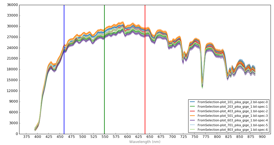
Notice that there is a range in radiance values across the various reference panels (e.g., the radiance in the green region ranges from ~26k to ~28k μW sr-1 cm-2 μm-1).
Note: The following example will load in several small hyperspectral radiance datacubes (not reflectance) that were previously cropped manually (via Spectronon software). These datacubes represent the radiance values of grey reference panels that were placed in the field to provide data necessary for converting radiance imagery to reflectance. These particular datacubes were extracted from several different images captured within ~10 minutes of each other.
Load and initialize the batch module, checking to be sure the directory exists.
[20]:
import os
from hs_process import batch

base_dir = os.path.join(data_dir, 'cube_ref_panels')
print(os.path.isdir(base_dir))
hsbatch = batch(base_dir)
True
Combine all the radiance datacubes in the directory via batch.spectra_combine.
[21]:
hsbatch.spectra_combine(base_dir=base_dir, search_ext='bip', dir_level=0, out_force=True)
Combining datacubes/spectra into a single mean spectra.
Number of input datacubes/spectra: 7
Total number of pixels: 1516
Visualize the combined spectra by opening in Spectronon. The solid line represents the mean radiance spectra across all pixels and images in base_dir, and the lighter, slightly transparent line represents the standard deviation of the radiance across all pixels and images in base_dir.
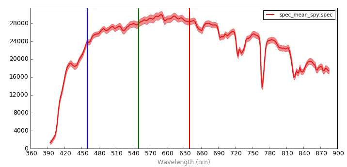
Notice the lower signal at the oxygen absorption region (near 770 nm). After converting datacubes to reflectance, it may be desireable to spectrally clip this region (see `spec_mod.spectral_clip <tutorial_spec_mod.html#spec_mod.spectral_clip>`__)
7.9. batch.spectra_to_csv
Reads all the .spec files in a direcory and saves their reflectance information to a .csv. batch.spectra_to_csv is identical to batch.spectra_to_df except a .csv file is saved rather than returning a pandas.DataFrame. [API]
Note: The following example builds on the results of the `batch.segment_band_math tutorial <tutorial_batch.html#batch.segment_band_math>`__ and `batch.segment_create_mask <tutorial_batch.html#batch.segment_create_mask>`__. Please complete each of those tutorial examples to be sure your directory (i.e., F:\\nigo0024\Documents\hs_process_demo\spatial_mod\crop_many_gdf\mask_mcari2_90th) is populated with image files.
Load and initialize the batch module, checking to be sure the directory exists.
[22]:
import os
from hs_process import batch

base_dir = os.path.join(data_dir, 'spatial_mod', 'crop_many_gdf', 'mask_mcari2_90th')
print(os.path.isdir(base_dir))
hsbatch = batch(base_dir)
True
Read all the .spec files in base_dir and save them to a .csv file.
[23]:
hsbatch.spectra_to_csv(base_dir=base_dir, search_ext='spec', dir_level=0)
Writing mean spectra to a .csv file.
Number of input datacubes/spectra: 40
Output file location: F:\\nigo0024\Documents\hs_process_demo\spatial_mod\crop_many_gdf\mask_mcari2_90th\stats-spectra.csv
When stats-spectra.csv is opened, we can see that each row is a .spec file from a different plot, and each column is a particular spectral band/wavelength.
[24]:
import pandas as pd
pd.read_csv(os.path.join(base_dir, 'stats-spectra.csv')).head(5)
[24]:
| Unnamed: 0 | wavelength | 394.6 | 396.6528 | 398.7056 | 400.7584 | 402.8112 | 404.864 | 406.9168 | 408.9696 | ... | 866.744 | 868.7968 | 870.8496 | 872.9024 | 874.9552 | 877.008 | 879.0608 | 881.1136 | 883.1664 | 885.2192 | |
|---|---|---|---|---|---|---|---|---|---|---|---|---|---|---|---|---|---|---|---|---|---|
| 0 | fname | plot_id | 1.000000 | 2.000000 | 3.000000 | 4.000000 | 5.000000 | 6.000000 | 7.000000 | 8.000000 | ... | 231.000000 | 232.000000 | 233.000000 | 234.000000 | 235.000000 | 236.000000 | 237.000000 | 238.000000 | 239.000000 | 240.000000 |
| 1 | Wells_rep2_20180628_16h56m_pika_gige_7_plot_10... | 1011 | 13.523563 | 19.213570 | 9.585402 | 7.049162 | 4.971103 | 3.669440 | 2.547665 | 1.944489 | ... | 45.952736 | 45.177956 | 44.178223 | 45.595730 | 44.237053 | 45.192883 | 44.707069 | 44.317673 | 44.977257 | 44.885410 |
| 2 | Wells_rep2_20180628_16h56m_pika_gige_7_plot_10... | 1012 | 14.328226 | 17.673107 | 9.557288 | 6.861992 | 5.470718 | 4.297456 | 2.747330 | 2.122929 | ... | 44.907276 | 44.544106 | 43.384926 | 44.675610 | 43.880154 | 44.394325 | 43.728794 | 43.444515 | 44.277538 | 44.192337 |
| 3 | Wells_rep2_20180628_16h56m_pika_gige_7_plot_10... | 1013 | 13.280209 | 18.991058 | 9.806862 | 7.041559 | 5.084080 | 4.054595 | 2.607378 | 2.187212 | ... | 40.590130 | 40.234657 | 39.194435 | 40.260246 | 39.648201 | 40.096077 | 39.318855 | 39.217598 | 39.904327 | 39.873375 |
| 4 | Wells_rep2_20180628_16h56m_pika_gige_7_plot_10... | 1014 | 12.916803 | 18.932661 | 9.879722 | 6.712576 | 4.815042 | 3.865411 | 2.757464 | 2.130761 | ... | 46.262978 | 45.802395 | 44.400795 | 45.824875 | 45.436096 | 45.664883 | 44.691391 | 44.591335 | 45.321087 | 45.260036 |
5 rows × 242 columns
7.10. batch.spectra_to_df
Reads all the .spec files in a direcory and returns their data as a pandas.DataFrame object. batch.spectra_to_df is identical to batch.spectra_to_csv except a pandas.DataFrame is returned rather than saving a .csv file. [API]
Note: The following example builds on the results of the `batch.segment_band_math tutorial <tutorial_batch.html#batch.segment_band_math>`__ and `batch.segment_create_mask <tutorial_batch.html#batch.segment_create_mask>`__. Please complete each of those tutorial examples to be sure your directory (i.e., F:\\nigo0024\Documents\hs_process_demo\spatial_mod\crop_many_gdf\mask_mcari2_90th) is populated with image files.
Load and initialize the batch module, checking to be sure the directory exists.
[25]:
import os
from hs_process import batch

base_dir = os.path.join(data_dir, 'spatial_mod', 'crop_many_gdf', 'mask_mcari2_90th')
print(os.path.isdir(base_dir))
hsbatch = batch(base_dir)
True
Read all the .spec files in base_dir and load them to df_spec, a pandas.DataFrame.
[26]:
df_spec = hsbatch.spectra_to_df(base_dir=base_dir, search_ext='spec', dir_level=0)
df_spec.head(5)
Writing mean spectra to a ``pandas.DataFrame``.
Number of input datacubes/spectra: 40
[26]:
| fname | plot_id | 1 | 2 | 3 | 4 | 5 | 6 | 7 | 8 | ... | 231 | 232 | 233 | 234 | 235 | 236 | 237 | 238 | 239 | 240 | |
|---|---|---|---|---|---|---|---|---|---|---|---|---|---|---|---|---|---|---|---|---|---|
| 0 | Wells_rep2_20180628_16h56m_pika_gige_7_plot_10... | 1011 | 13.523563 | 19.213570 | 9.585402 | 7.049162 | 4.971103 | 3.669440 | 2.547665 | 1.944489 | ... | 45.952736 | 45.177956 | 44.178223 | 45.595730 | 44.237053 | 45.192883 | 44.707069 | 44.317673 | 44.977257 | 44.885410 |
| 1 | Wells_rep2_20180628_16h56m_pika_gige_7_plot_10... | 1012 | 14.328226 | 17.673107 | 9.557288 | 6.861992 | 5.470718 | 4.297456 | 2.747330 | 2.122929 | ... | 44.907276 | 44.544106 | 43.384926 | 44.675610 | 43.880154 | 44.394325 | 43.728794 | 43.444515 | 44.277538 | 44.192337 |
| 2 | Wells_rep2_20180628_16h56m_pika_gige_7_plot_10... | 1013 | 13.280209 | 18.991058 | 9.806862 | 7.041559 | 5.084080 | 4.054595 | 2.607378 | 2.187212 | ... | 40.590130 | 40.234657 | 39.194435 | 40.260246 | 39.648201 | 40.096077 | 39.318855 | 39.217598 | 39.904327 | 39.873375 |
| 3 | Wells_rep2_20180628_16h56m_pika_gige_7_plot_10... | 1014 | 12.916803 | 18.932661 | 9.879722 | 6.712576 | 4.815042 | 3.865411 | 2.757464 | 2.130761 | ... | 46.262978 | 45.802395 | 44.400795 | 45.824875 | 45.436096 | 45.664883 | 44.691391 | 44.591335 | 45.321087 | 45.260036 |
| 4 | Wells_rep2_20180628_16h56m_pika_gige_7_plot_10... | 1015 | 12.629728 | 20.137224 | 9.565381 | 6.610282 | 5.238615 | 4.095292 | 2.672005 | 2.190024 | ... | 46.753952 | 46.385578 | 44.936142 | 46.200020 | 45.938831 | 46.119297 | 45.290573 | 45.130165 | 45.812798 | 45.785793 |
5 rows × 242 columns
Each row is a .spec file from a different plot, and each column is a particular spectral band.
It is somewhat confusing to conceptualize spectral data by band number (as opposed to the wavelenth it represents). hs_process.hs_tools.get_band can be used to retrieve spectral data for all plots via indexing by wavelength. Say we need to access reflectance at 710 nm for each plot (in this case, the 710 nm band is band number 155).
[27]:
df_710nm = df_spec[['fname', 'plot_id', hsbatch.io.tools.get_band(710)]]
df_710nm.head(5)
[27]:
| fname | plot_id | 155 | |
|---|---|---|---|
| 0 | Wells_rep2_20180628_16h56m_pika_gige_7_plot_10... | 1011 | 5.769057 |
| 1 | Wells_rep2_20180628_16h56m_pika_gige_7_plot_10... | 1012 | 6.112481 |
| 2 | Wells_rep2_20180628_16h56m_pika_gige_7_plot_10... | 1013 | 6.855353 |
| 3 | Wells_rep2_20180628_16h56m_pika_gige_7_plot_10... | 1014 | 6.578203 |
| 4 | Wells_rep2_20180628_16h56m_pika_gige_7_plot_10... | 1015 | 6.886356 |
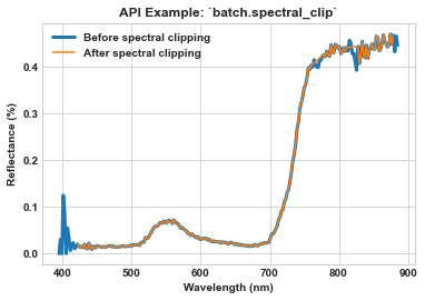
7.11. batch.spectral_clip
Batch processing tool to spectrally clip multiple datacubes in the same way. [API]
Note: The following example builds on the results of the `batch.spatial_crop tutorial <tutorial_batch.html#batch.spatial_crop>`__. Please complete the batch.spatial_crop tutorial example to be sure your directory (i.e., base_dir) is populated with multiple hyperspectral datacubes. The following example will be using datacubes located in teh following directory: F:\\nigo0024\Documents\hs_process_demo\spatial_crop
Load and initialize the batch module, checking to be sure the directory exists.
[28]:
import os
from hs_process import batch

base_dir = os.path.join(data_dir, 'spatial_crop')
print(os.path.isdir(base_dir))
hsbatch = batch(base_dir, search_ext='.bip',
                progress_bar=True)  # searches for all files in ``base_dir`` with a ".bip" file extension
True
Use batch.spectral_clip to clip all spectral bands below 420 nm and above 880 nm, as well as the bands near the oxygen absorption (i.e., 760-776 nm) and water absorption (i.e., 813-827 nm) regions.
[29]:
hsbatch.spectral_clip(base_dir=base_dir, folder_name='spec_clip',
                      wl_bands=[[0, 420], [760, 776], [813, 827], [880, 1000]],
                      out_force=True)
Processing file 79/80: 100%|████████████████████████████████████████████████████████████████████| 80/80 [00:03<00:00, 20.77it/s]
Use Seaborn to visualize the spectra of a single pixel in one of the processed images.
[30]:
import seaborn as sns

fname = os.path.join(base_dir, 'Wells_rep2_20180628_16h56m_pika_gige_7_plot_1011-spatial-crop.bip')
hsbatch.io.read_cube(fname)
spy_mem = hsbatch.io.spyfile.open_memmap()  # datacube before clipping
meta_bands = list(hsbatch.io.tools.meta_bands.values())
fname = os.path.join(base_dir, 'spec_clip', 'Wells_rep2_20180628_16h56m_pika_gige_7_plot_1011-spec-clip.bip')
hsbatch.io.read_cube(fname)
spy_mem_clip = hsbatch.io.spyfile.open_memmap()  # datacube after clipping
meta_bands_clip = list(hsbatch.io.tools.meta_bands.values())
ax = sns.lineplot(x=meta_bands, y=spy_mem[26][29], label='Before spectral clipping', linewidth=3)
ax = sns.lineplot(x=meta_bands_clip, y=spy_mem_clip[26][29], label='After spectral clipping', ax=ax)
ax.set_xlabel('Wavelength (nm)', weight='bold')
ax.set_ylabel('Reflectance (%)', weight='bold')
ax.set_title(r'API Example: `batch.spectral_clip`', weight='bold')
[30]:
Text(0.5, 1.0, 'API Example: `batch.spectral_clip`')
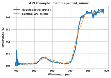
7.12. batch.spectral_mimic
Batch processing tool to spectrally mimic a multispectral sensor for multiple datacubes in the same way. [API]
Note: The following example builds on the results of the batch.spatial_crop tutorial. Please complete the batch.spatial_crop tutorial example to be sure your directory (i.e., base_dir) is populated with multiple hyperspectral datacubes. The following example will be using datacubes located in the following directory: F:\\nigo0024\Documents\hs_process_demo\spatial_crop
Load and initialize the batch module, checking to be sure the directory exists.
[31]:
import os
from hs_process import batch

base_dir = os.path.join(data_dir, 'spatial_crop')
print(os.path.isdir(base_dir))
hsbatch = batch(base_dir, search_ext='.bip', progress_bar=True)  # searches for all files in ``base_dir`` with a ".bip" file extension
True
Use batch.spectral_mimic to spectrally mimic the Sentinel-2A multispectral satellite sensor.
[32]:
hsbatch.spectral_mimic(base_dir=base_dir, folder_name='spec_mimic',
                       name_append='sentinel-2a',
                       sensor='sentinel-2a', center_wl='weighted',
                       out_force=True)
Processing file 79/80: 100%|████████████████████████████████████████████████████████████████████| 80/80 [00:08<00:00, 9.42it/s]
Use seaborn to visualize the spectra of a single pixel in one of the processed images.
[33]:
import seaborn as sns
fname = os.path.join(base_dir, 'Wells_rep2_20180628_16h56m_pika_gige_7_plot_1011-spatial-crop.bip')
hsbatch.io.read_cube(fname)
spy_mem = hsbatch.io.spyfile.open_memmap()  # datacube before mimicking
meta_bands = list(hsbatch.io.tools.meta_bands.values())
fname = os.path.join(base_dir, 'spec_mimic', 'Wells_rep2_20180628_16h56m_pika_gige_7_plot_1011-sentinel-2a.bip')
hsbatch.io.read_cube(fname)
spy_mem_sen2a = hsbatch.io.spyfile.open_memmap()  # datacube after mimicking
meta_bands_sen2a = list(hsbatch.io.tools.meta_bands.values())
ax = sns.lineplot(x=meta_bands, y=spy_mem[26][29], label='Hyperspectral (Pika II)', linewidth=3)
ax = sns.lineplot(x=meta_bands_sen2a, y=spy_mem_sen2a[26][29], label='Sentinel-2A "mimic"', marker='o', ms=6, ax=ax)
ax.set_xlabel('Wavelength (nm)', weight='bold')
ax.set_ylabel('Reflectance (%)', weight='bold')
ax.set_title(r'API Example: `batch.spectral_mimic`', weight='bold')
[33]:
Text(0.5, 1.0, 'API Example: `batch.spectral_mimic`')
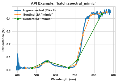
Use spec_mod.spectral_mimic to mimic the Sentera 6x spectral configuration and compare to both hyperspectral and Sentinel-2A.
[34]:
hsbatch.spectral_mimic(base_dir=base_dir, folder_name='spec_mimic',
                       name_append='sentera-6x',
                       sensor='sentera_6x', center_wl='weighted',
                       out_force=True)

fname = os.path.join(base_dir, 'spec_mimic', 'Wells_rep2_20180628_16h56m_pika_gige_7_plot_1011-sentera-6x.bip')
hsbatch.io.read_cube(fname)
spy_mem_6x = hsbatch.io.spyfile.open_memmap()  # datacube after mimicking
meta_bands_6x = list(hsbatch.io.tools.meta_bands.values())
ax = sns.lineplot(x=meta_bands, y=spy_mem[26][29], label='Hyperspectral (Pika II)', linewidth=3)
ax = sns.lineplot(x=meta_bands_sen2a, y=spy_mem_sen2a[26][29], label='Sentinel-2A "mimic"', marker='o', ms=6, ax=ax)
ax = sns.lineplot(x=meta_bands_6x, y=spy_mem_6x[26][29], label='Sentera 6X "mimic"', color='green', marker='o', ms=8, ax=ax)
ax.set_xlabel('Wavelength (nm)', weight='bold')
ax.set_ylabel('Reflectance (%)', weight='bold')
ax.set_title(r'API Example: `batch.spectral_mimic`', weight='bold')
Processing file 79/80: 100%|████████████████████████████████████████████████████████████████████| 80/80 [00:05<00:00, 14.79it/s]
[34]:
Text(0.5, 1.0, 'API Example: `batch.spectral_mimic`')
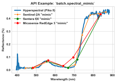
And finally, mimic the Micasense RedEdge-MX and compare to hyperspectral, Sentinel-2A, and Sentera 6X.
[35]:
hsbatch.spectral_mimic(base_dir=base_dir, folder_name='spec_mimic',
                       name_append='micasense-rededge-3',
                       sensor='micasense_rededge_3', center_wl='weighted',
                       out_force=True)

fname = os.path.join(base_dir, 'spec_mimic', 'Wells_rep2_20180628_16h56m_pika_gige_7_plot_1011-micasense-rededge-3.bip')
hsbatch.io.read_cube(fname)
spy_mem_re3 = hsbatch.io.spyfile.open_memmap()  # datacube after mimicking
meta_bands_re3 = list(hsbatch.io.tools.meta_bands.values())
ax = sns.lineplot(x=meta_bands, y=spy_mem[26][29], label='Hyperspectral (Pika II)', linewidth=3)
ax = sns.lineplot(x=meta_bands_sen2a, y=spy_mem_sen2a[26][29], label='Sentinel-2A "mimic"', marker='o', ms=6, ax=ax)
ax = sns.lineplot(x=meta_bands_6x, y=spy_mem_6x[26][29], label='Sentera 6X "mimic"', color='green', marker='o', ms=8, ax=ax)
ax = sns.lineplot(x=meta_bands_re3, y=spy_mem_re3[26][29], label='Micasense RedEdge 3 "mimic"', color='red', marker='o', ms=8, ax=ax)
ax.set_xlabel('Wavelength (nm)', weight='bold')
ax.set_ylabel('Reflectance (%)', weight='bold')
ax.set_title(r'API Example: `batch.spectral_mimic`', weight='bold')
Processing file 79/80: 100%|████████████████████████████████████████████████████████████████████| 80/80 [00:05<00:00, 15.25it/s]
[35]:
Text(0.5, 1.0, 'API Example: `batch.spectral_mimic`')
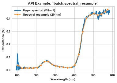
7.13. batch.spectral_resample
Batch processing tool to spectrally resample (a.k.a. “bin”) multiple datacubes in the same way. [API]
Note: The following example builds on the results of the batch.spatial_crop tutorial. Please complete the batch.spatial_crop tutorial example to be sure your directory (i.e., base_dir) is populated with multiple hyperspectral datacubes. The following example will be using datacubes located in the following directory: F:\\nigo0024\Documents\hs_process_demo\spatial_crop
Load and initialize the batch module, checking to be sure the directory exists.
[36]:
import os
from hs_process import batch

base_dir = os.path.join(data_dir, 'spatial_crop')
print(os.path.isdir(base_dir))
hsbatch = batch(base_dir, search_ext='.bip', progress_bar=True)  # searches for all files in ``base_dir`` with a ".bip" file extension
True
Use batch.spectral_resample to bin (a.k.a., “group”) all spectral bands into 20 nm bandwidth bands (from ~2.3 nm bandwidth originally) on a per-pixel basis.
[37]:
hsbatch.spectral_resample(base_dir=base_dir, folder_name='spec_bin',
                          name_append='spec-bin-20',
                          bandwidth=20, out_force=True)
Processing file 79/80: 100%|████████████████████████████████████████████████████████████████████| 80/80 [00:01<00:00, 55.82it/s]
Use seaborn to visualize the spectra of a single pixel in one of the processed images.
[38]:
import seaborn as sns
fname = os.path.join(base_dir, 'Wells_rep2_20180628_16h56m_pika_gige_7_plot_1011-spatial-crop.bip')
hsbatch.io.read_cube(fname)
spy_mem = hsbatch.io.spyfile.open_memmap()  # datacube before resampling
meta_bands = list(hsbatch.io.tools.meta_bands.values())
fname = os.path.join(base_dir, 'spec_bin', 'Wells_rep2_20180628_16h56m_pika_gige_7_plot_1011-spec-bin-20.bip')
hsbatch.io.read_cube(fname)
spy_mem_bin = hsbatch.io.spyfile.open_memmap()  # datacube after resampling
meta_bands_bin = list(hsbatch.io.tools.meta_bands.values())
ax = sns.lineplot(x=meta_bands, y=spy_mem[26][29], label='Hyperspectral (Pika II)', linewidth=3)
ax = sns.lineplot(x=meta_bands_bin, y=spy_mem_bin[26][29], label='Spectral resample (20 nm)', marker='o', ms=6, ax=ax)
ax.set_xlabel('Wavelength (nm)', weight='bold')
ax.set_ylabel('Reflectance (%)', weight='bold')
ax.set_title(r'API Example: `batch.spectral_resample`', weight='bold')
[38]:
Text(0.5, 1.0, 'API Example: `batch.spectral_resample`')
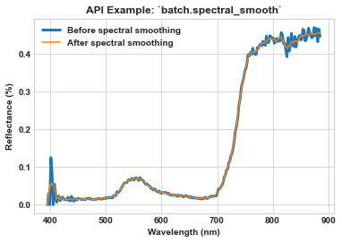
7.14. batch.spectral_smooth
Batch processing tool to spectrally smooth multiple datacubes in the same way. [API]
Note: The following example builds on the results of the batch.spatial_crop tutorial. Please complete the batch.spatial_crop tutorial example to be sure your directory (i.e., base_dir) is populated with multiple hyperspectral datacubes. The following example will be using datacubes located in the following directory: F:\\nigo0024\Documents\hs_process_demo\spatial_crop
Load and initialize the batch module, checking to be sure the directory exists.
[39]:
import os
from hs_process import batch

base_dir = os.path.join(data_dir, 'spatial_crop')
print(os.path.isdir(base_dir))
hsbatch = batch(base_dir, search_ext='.bip', progress_bar=True)  # searches for all files in ``base_dir`` with a ".bip" file extension
True
Use batch.spectral_smooth to perform a Savitzky-Golay smoothing operation on each image/pixel in base_dir. The window_size and order can be adjusted to achieve desired smoothing results.
[40]:
hsbatch.spectral_smooth(base_dir=base_dir, folder_name='spec_smooth',
                        window_size=11, order=2, out_force=True)
Processing file 79/80: 100%|████████████████████████████████████████████████████████████████████| 80/80 [02:01<00:00, 1.52s/it]
Use Seaborn to visualize the spectra of a single pixel in one of the processed images.
[41]:
import seaborn as sns

fname = os.path.join(base_dir, 'Wells_rep2_20180628_16h56m_pika_gige_7_plot_1011-spatial-crop.bip')
hsbatch.io.read_cube(fname)
spy_mem = hsbatch.io.spyfile.open_memmap()  # datacube before smoothing
meta_bands = list(hsbatch.io.tools.meta_bands.values())
fname = os.path.join(base_dir, 'spec_smooth', 'Wells_rep2_20180628_16h56m_pika_gige_7_plot_1011-spec-smooth.bip')
hsbatch.io.read_cube(fname)
spy_mem_clip = hsbatch.io.spyfile.open_memmap()  # datacube after smoothing
meta_bands_clip = list(hsbatch.io.tools.meta_bands.values())
ax = sns.lineplot(x=meta_bands, y=spy_mem[26][29], label='Before spectral smoothing', linewidth=3)
ax = sns.lineplot(x=meta_bands_clip, y=spy_mem_clip[26][29], label='After spectral smoothing', ax=ax)
ax.set_xlabel('Wavelength (nm)', weight='bold')
ax.set_ylabel('Reflectance (%)', weight='bold')
ax.set_title(r'API Example: `batch.spectral_smooth`', weight='bold')
[41]:
Text(0.5, 1.0, 'API Example: `batch.spectral_smooth`')