5. Tutorial: spec_mod
5.1. Sample data
Sample imagery captured from a Resonon Pika II VIS-NIR line scanning imager and ancillary sample files can be downloaded from this link.
Before trying this tutorial on your own machine, please download the sample files and place into a local directory of your choosing (and do not change the file names). Indicate the location of your sample files by modifying data_dir:
[1]:
data_dir = r'F:\\nigo0024\Documents\hs_process_demo'
5.2. Confirm your environment
Before trying the tutorials, be sure hs_process and its dependencies are properly installed. If you installed in a virtual environment, first check we are indeed using the Python instance that was installed with the virtual environment:
[2]:
import sys
import hs_process
print('Python install location: {0}'.format(sys.executable))
print('Version: {0}'.format(hs_process.__version__))
Python install location: C:\Users\nigo0024\Anaconda3\envs\hs_process\python.exe
Version: 0.0.4
The spec folder that contains python.exe tells me that the activated Python instance is indeed in the spec environment, just as I intend. If you created a virtual environment, but your python.exe is not in the envs\spec directory, you either did not properly create your virtual environment or you are not pointing to the correct Python installation in your IDE (e.g., Spyder, Jupyter notebook, etc.).
5.3. spec_mod.load_spyfile
Loads a SpyFile (Spectral Python object) for data access and/or manipulation by the hstools class. [API]
Load and initialize the hsio and spec_mod modules
[3]:
import os
from hs_process import hsio
from hs_process import spec_mod

fname_in = os.path.join(data_dir, 'Wells_rep2_20180628_16h56m_pika_gige_7-Radiance Conversion-Georectify Airborne Datacube-Convert Radiance Cube to Reflectance from Measured Reference Spectrum.bip.hdr')
io = hsio(fname_in)
my_spec_mod = spec_mod(io.spyfile)
Load datacube using spec_mod.load_spyfile
[4]:
my_spec_mod.load_spyfile(io.spyfile)
my_spec_mod.spyfile
[4]:
        Data Source:   'F:\\nigo0024\Documents\hs_process_demo\Wells_rep2_20180628_16h56m_pika_gige_7-Radiance Conversion-Georectify Airborne Datacube-Convert Radiance Cube to Reflectance from Measured Reference Spectrum.bip'
        # Rows:            617
        # Samples:        1300
        # Bands:           240
        Interleave:        BIP
        Quantization:  32 bits
        Data format:   float32
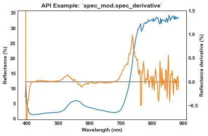
5.4. spec_mod.spec_derivative
Calculates the numeric derivative spectra from spyfile_spec. [API]
Load and initialize hsio
[5]:
import os
from hs_process import hsio
from hs_process import spec_mod
fname_hdr_spec = os.path.join(data_dir, 'Wells_rep2_20180628_16h56m_pika_gige_7_plot_611-cube-to-spec-mean.spec.hdr')
io = hsio()
io.read_spec(fname_hdr_spec)
my_spec_mod = spec_mod(io.spyfile_spec)
Calculate the numeric derivative.
[6]:
spec_dydx, metadata_dydx = my_spec_mod.spec_derivative(io.spyfile_spec) # Be sure this is the spec spyfile and not a full array
Plot the numeric derivative spectra and compare against the original spectra.
[7]:
import numpy as np
import seaborn as sns
sns.set_style("ticks")
wl_x = np.array([float(i) for i in metadata_dydx['wavelength']])
y_ref = io.spyfile_spec.open_memmap()[0,0,:]*100
ax1 = sns.lineplot(x=wl_x, y=y_ref)
ax2 = ax1.twinx()
ax2 = sns.lineplot(x=wl_x, y=0, ax=ax2, color='gray')
ax2 = sns.lineplot(x=wl_x, y=spec_dydx[0,0,:]*100, ax=ax2, color=sns.color_palette()[1])
ax2.set(ylim=(-0.8, 1.5))
ax1.set_xlabel('Wavelength (nm)', weight='bold')
ax1.set_ylabel('Reflectance (%)', weight='bold')
ax2.set_ylabel('Reflectance derivative (%)', weight='bold')
ax1.set_title(r'API Example: `spec_mod.spec_derivative`', weight='bold')
[7]:
Text(0.5, 1.0, 'API Example: `spec_mod.spec_derivative`')
Save the derivative spectra to file.
[8]:
fname_spec_der = os.path.join(data_dir, 'spec_mod', 'Wells_rep2_20180628_16h56m_pika_gige_7_plot_611-spec-derivative.spec.hdr')
io.write_spec(fname_spec_der, spec_dydx, df_std=None, metadata=metadata_dydx, force=True)
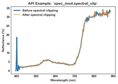
5.5. spec_mod.spectral_clip
Removes/clips designated wavelength bands from the hyperspectral datacube. [API]
Load and initialize the hsio and spec_mod modules
[9]:
import os
from hs_process import hsio
from hs_process import spec_mod

fname_hdr = os.path.join(data_dir, 'Wells_rep2_20180628_16h56m_pika_gige_7-Radiance Conversion-Georectify Airborne Datacube-Convert Radiance Cube to Reflectance from Measured Reference Spectrum.bip.hdr')
io = hsio()
io.read_cube(fname_hdr)
my_spec_mod = spec_mod(io.spyfile)
Using spec_mod.spectral_clip, clip all spectral bands below 420 nm and above 880 nm, as well as the bands near the oxygen absorption (i.e., 760-776 nm) and water absorption (i.e., 813-827 nm) regions.
[10]:
array_clip, metadata_clip = my_spec_mod.spectral_clip(wl_bands=[[0, 420], [760, 776], [813, 827], [880, 1000]])
Plot the spectra of the unclippe hyperspectral image and compare to that of the clipped image for a single pixel.
[11]:
import seaborn as sns
from ast import literal_eval

spy_hs = my_spec_mod.spyfile.open_memmap()  # datacube before smoothing
meta_bands = list(io.tools.meta_bands.values())
meta_bands_clip = sorted([float(i) for i in literal_eval(metadata_clip['wavelength'])])

ax = sns.lineplot(x=meta_bands, y=spy_hs[200][800]*100, label='Before spectral clipping', linewidth=3)
ax = sns.lineplot(x=meta_bands_clip, y=array_clip[200][800]*100, label='After spectral clipping', ax=ax)
ax.set_xlabel('Wavelength (nm)', weight='bold')
ax.set_ylabel('Reflectance (%)', weight='bold')
ax.set_title(r'API Example: `spec_mod.spectral_clip`', weight='bold')
[11]:
Text(0.5, 1.0, 'API Example: `spec_mod.spectral_clip`')
Save the clipped datacube
[12]:
from pathlib import Path

Path(os.path.join(data_dir, 'spec_mod')).mkdir(parents=True, exist_ok=True)
fname_hdr_clip = os.path.join(data_dir, 'spec_mod', 'Wells_rep2_20180628_16h56m_pika_gige_7-clip.bip.hdr')
io.write_cube(fname_hdr_clip, array_clip, metadata_clip, force=True)
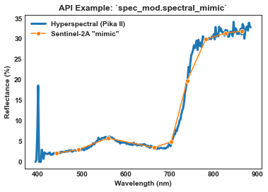
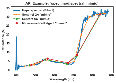
5.6. spec_mod.spectral_mimic
Mimics the response of a multispectral sensor based on transmissivity of sensor bands across a range of wavelength values by calculating its weighted average response and interpolating the hyperspectral response. [API]
Load and initialize the hsio and spec_mod modules
[13]:
import os
from hs_process import hsio
from hs_process import spec_mod

fname_hdr = os.path.join(data_dir, 'Wells_rep2_20180628_16h56m_pika_gige_7-Radiance Conversion-Georectify Airborne Datacube-Convert Radiance Cube to Reflectance from Measured Reference Spectrum.bip.hdr')
io = hsio()
io.read_cube(fname_hdr)

my_spec_mod = spec_mod(io.spyfile)
Use spec_mod.spectral_mimic to mimic the Sentinel-2A spectral response function.
[14]:
array_s2a, metadata_s2a = my_spec_mod.spectral_mimic(sensor='sentinel-2a', center_wl='weighted')
Plot the spectra of the hyperspectral image and compare to that of the mimicked Sentinel-2A for a single pixel.
[15]:
import seaborn as sns

spy_hs = my_spec_mod.spyfile.open_memmap()  # datacube before smoothing
meta_bands = list(io.tools.meta_bands.values())
meta_bands_s2a = sorted([float(i) for i in literal_eval(metadata_s2a['wavelength'])])

ax = sns.lineplot(x=meta_bands, y=spy_hs[200][800]*100, label='Hyperspectral (Pika II)', linewidth=3)
ax = sns.lineplot(x=meta_bands_s2a, y=array_s2a[200][800]*100, label='Sentinel-2A "mimic"', marker='o', ms=6, ax=ax)
ax.set_xlabel('Wavelength (nm)', weight='bold')
ax.set_ylabel('Reflectance (%)', weight='bold')
ax.set_title(r'API Example: `spec_mod.spectral_mimic`', weight='bold')
[15]:
Text(0.5, 1.0, 'API Example: `spec_mod.spectral_mimic`')
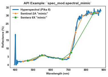
Use spec_mod.spectral_mimic to mimic the Sentera 6x spectral configuration and compare to both hyperspectral and Sentinel-2A.
[16]:
array_6x, metadata_6x = my_spec_mod.spectral_mimic(sensor='sentera_6x', center_wl='peak')
meta_bands_6x = sorted([float(i) for i in literal_eval(metadata_6x['wavelength'])])

ax = sns.lineplot(x=meta_bands, y=spy_hs[200][800]*100, label='Hyperspectral (Pika II)', linewidth=3)
ax = sns.lineplot(x=meta_bands_s2a, y=array_s2a[200][800]*100, label='Sentinel-2A "mimic"', marker='o', ms=6, ax=ax)
ax = sns.lineplot(x=meta_bands_6x, y=array_6x[200][800]*100, label='Sentera 6X "mimic"', marker='o', ms=8, ax=ax)
ax.set_xlabel('Wavelength (nm)', weight='bold')
ax.set_ylabel('Reflectance (%)', weight='bold')
ax.set_title(r'API Example: `spec_mod.spectral_mimic`', weight='bold')
[16]:
Text(0.5, 1.0, 'API Example: `spec_mod.spectral_mimic`')
And finally, mimic the Micasense RedEdge-MX and compare to hyperspectral, Sentinel-2A, and Sentera 6X.
[17]:
array_re3, metadata_re3 = my_spec_mod.spectral_mimic(sensor='micasense_rededge_3', center_wl='peak')
meta_bands_re3 = sorted([float(i) for i in literal_eval(metadata_re3['wavelength'])])

ax = sns.lineplot(x=meta_bands, y=spy_hs[200][800]*100, label='Hyperspectral (Pika II)', linewidth=3)
ax = sns.lineplot(x=meta_bands_s2a, y=array_s2a[200][800]*100, label='Sentinel-2A "mimic"', marker='o', ms=6, ax=ax)
ax = sns.lineplot(x=meta_bands_6x, y=array_6x[200][800]*100, label='Sentera 6X "mimic"', marker='o', ms=8, ax=ax)
ax = sns.lineplot(x=meta_bands_re3, y=array_re3[200][800]*100, label='Micasense RedEdge 3 "mimic"', marker='o', ms=8, ax=ax)
ax.set_xlabel('Wavelength (nm)', weight='bold')
ax.set_ylabel('Reflectance (%)', weight='bold')
ax.set_title(r'API Example: `spec_mod.spectral_mimic`', weight='bold')
[17]:
Text(0.5, 1.0, 'API Example: `spec_mod.spectral_mimic`')
Save the mimicked datacubes using hsio.write_cube
[18]:
fname_hdr_mimic_s2a = os.path.join(data_dir, 'spec_mod', 'Wells_rep2_20180628_16h56m_pika_gige_7-mimic-s2a.bip.hdr')
fname_hdr_mimic_6x = os.path.join(data_dir, 'spec_mod', 'Wells_rep2_20180628_16h56m_pika_gige_7-mimic-6x.bip.hdr')
fname_hdr_mimic_re3 = os.path.join(data_dir, 'spec_mod', 'Wells_rep2_20180628_16h56m_pika_gige_7-mimic-re3.bip.hdr')
io.write_cube(fname_hdr_mimic_s2a, array_s2a, metadata_s2a, force=True)
io.write_cube(fname_hdr_mimic_6x, array_6x, metadata_6x, force=True)
io.write_cube(fname_hdr_mimic_re3, array_re3, metadata_re3, force=True)
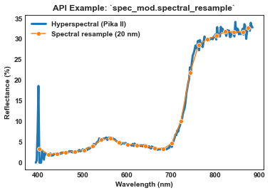
5.7. spec_mod.spectral_resample
Performs pixel-wise resampling of spectral bands via binning (calculates the mean across all bands within each bandwidth region for each image pixel). [API]
Load and initialize the hsio and spec_mod modules
[19]:
import os
from hs_process import hsio
from hs_process import spec_mod

fname_hdr = os.path.join(data_dir, 'Wells_rep2_20180628_16h56m_pika_gige_7-Radiance Conversion-Georectify Airborne Datacube-Convert Radiance Cube to Reflectance from Measured Reference Spectrum.bip.hdr')
io = hsio()
io.read_cube(fname_hdr)

my_spec_mod = spec_mod(io.spyfile)
Use spec_mod.spectral_resample to “bin” the datacube to bands with 20 nm bandwidths.
[20]:
array_bin, metadata_bin = my_spec_mod.spectral_resample(bandwidth=20)
Plot the spectra for both the hyperspectral image and that of the binned image bands (for a single “vegetation” pixel).
[21]:
import seaborn as sns
from ast import literal_eval

spy_hs = my_spec_mod.spyfile.open_memmap()  # datacube before smoothing
meta_bands = list(io.tools.meta_bands.values())
# meta_bands_bin = sorted([float(i) for i in metadata_bin['wavelength']])
meta_bands_bin = sorted([float(i) for i in literal_eval(metadata_bin['wavelength'])])

ax = sns.lineplot(x=meta_bands, y=spy_hs[200][800]*100, label='Hyperspectral (Pika II)', linewidth=3)
ax = sns.lineplot(x=meta_bands_bin, y=array_bin[200][800]*100, label='Spectral resample (20 nm)', marker='o', ms=6, ax=ax)
ax.set_xlabel('Wavelength (nm)', weight='bold')
ax.set_ylabel('Reflectance (%)', weight='bold')
ax.set_title(r'API Example: `spec_mod.spectral_resample`', weight='bold')
[21]:
Text(0.5, 1.0, 'API Example: `spec_mod.spectral_resample`')
Save the spectrally resampled datacube using hsio.write_cube
[22]:
fname_hdr_bin = os.path.join(data_dir, 'spec_mod', 'Wells_rep2_20180628_16h56m_pika_gige_7-bin-20.bip.hdr')
io.write_cube(fname_hdr_bin, array_bin, metadata_bin, force=True)
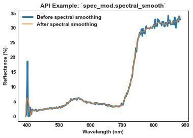
5.8. spec_mod.spectral_smooth
Performs Savitzky-Golay smoothing on the spectral domain. [API]
Load and initialize the hsio and spec_mod modules
[23]:
import os
from hs_process import hsio
from hs_process import spec_mod

fname_hdr = os.path.join(data_dir, 'Wells_rep2_20180628_16h56m_pika_gige_7-Radiance Conversion-Georectify Airborne Datacube-Convert Radiance Cube to Reflectance from Measured Reference Spectrum.bip.hdr')
io = hsio()
io.read_cube(fname_hdr)
my_spec_mod = spec_mod(io.spyfile)
Use spec_mod.spectral_smooth to perform a Savitzky-Golay smoothing operation across the hyperspectral spectral signature.
[24]:
array_smooth, metadata_smooth = my_spec_mod.spectral_smooth(window_size=11, order=2)
Plot the spectra of an individual pixel to visualize the result of the smoothing procedure.
[25]:
import seaborn as sns
from ast import literal_eval

spy_hs = my_spec_mod.spyfile.open_memmap()  # datacube before smoothing
meta_bands = list(io.tools.meta_bands.values())
meta_bands_smooth = sorted([float(i) for i in metadata_smooth['wavelength']])

ax = sns.lineplot(x=meta_bands, y=spy_hs[200][800]*100, label='Before spectral smoothing', linewidth=3)
ax = sns.lineplot(x=meta_bands_smooth, y=array_smooth[200][800]*100, label='After spectral smoothing', ax=ax)
ax.set_xlabel('Wavelength (nm)', weight='bold')
ax.set_ylabel('Reflectance (%)', weight='bold')
ax.set_title(r'API Example: `spec_mod.spectral_smooth`', weight='bold')
[25]:
Text(0.5, 1.0, 'API Example: `spec_mod.spectral_smooth`')
Save the smoothed datacube using hsio.write_cube
[26]:
fname_hdr_smooth = os.path.join(data_dir, 'spec_mod', 'Wells_rep2_20180628_16h56m_pika_gige_7-smooth.bip.hdr')
io.write_cube(fname_hdr_smooth, array_smooth, metadata_smooth, force=True)